What will be illustrated in this post is strongly in spired by the content of the books “Statistical Rethinking” (McElreath 2018) and “Bayesian Data Analysis 3rd Edition” (Gelman et al. 1995). In particular, the idea to separately code and illustrate the behavior of different covariance kernel functions comes from the amazing “Kernel Cookbook” and PhD thesis of David Duvenaud (Duvenaud 2014).
This post assumes some level of knowledge in bayesian statistics and probabilistic programming.
1.1 What we will cover
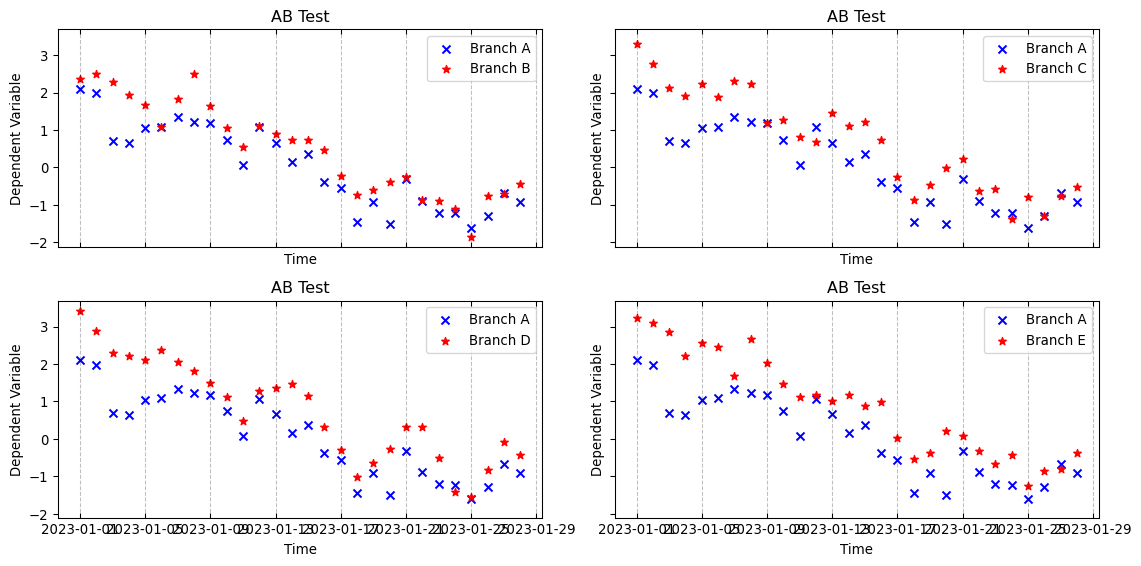
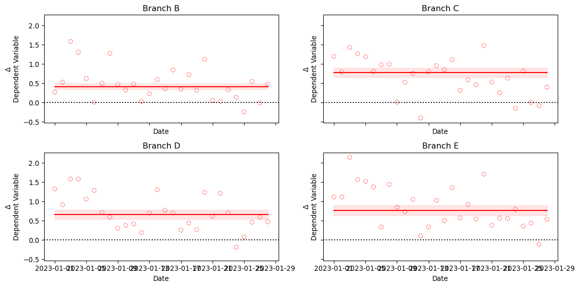
Very brief illustration of longitudinal A/B test within and observational paradigm.
Very brief illustration of gaussian processes and their application to analyzing A/B test data.
Overview of how to implement a gaussian process model using Numpyro and JAX.
Simulating A/B test data.
Analyzing A/B test data within an modelling setting.
1.2 What we will not cover
Detailed coverage of A/B test (e.g., sampling, randomization etc…).
Hypothesis testing (we will focus on modelling).
Fundamentals of bayesian statistics.
Detailed overview of Gaussian processes.
Probabilistic programming and sampling algorithms.
2 Introduction
2.1 Longitudinal A/B tests in observational settings
When we talk about A/B test we usually refer to a research method used for evaluating if a given intervention is having an impact on a pre-defined outcome variable measured inside a sample. For doing so, we can draw two distinct samples (the A and B group) from a population of interest, subject one of the two to the intervention and then measure observed differences in the outcome variable. Subject to several assumptions and pre-conditions (we suggest reading part V of “Regression and Other Stories” (Gelman, Hill, and Vehtari 2021)), if we observe a difference between the two groups when can conclude that our intervention might have had an impact on our outcome variable.
2.2 Gaussian Process
The Gaussian Process \(GP\) can be thought as the continuous generalization of basis function regression (see Chapter 20 of (Gelman et al. 1995)). We can think of it as a stochastic process where any point drawn from it, \(x_1, \dots, x_n\), comes from a multi-dimensional gaussian. In other words, it is as a prior distribution over an un-known function \(\mu(x)\) defined as
where \(m\) is a mean function and \(k\) is a covariance function. We can already have an intuition of how defining the \(GP\) in terms mean and covariance functions gives us quite some flexibility as it allows us to produce a model than can interpolate for all the value of \(x\).
The \(m\) function provides the most likely guess for the \(GP\) like the mean vector of a multi-dimensional Gaussian, deviation from this expected model are then handled by the covariance function \(k\).
The \(k\) function (often called Kernel) allows to structurally define the \(GP\) behavior at any two points by producing an \(n \times n\) covariance function given by evaluating \(k(x, x')\) for every \(x_1, \dots, x_n\).
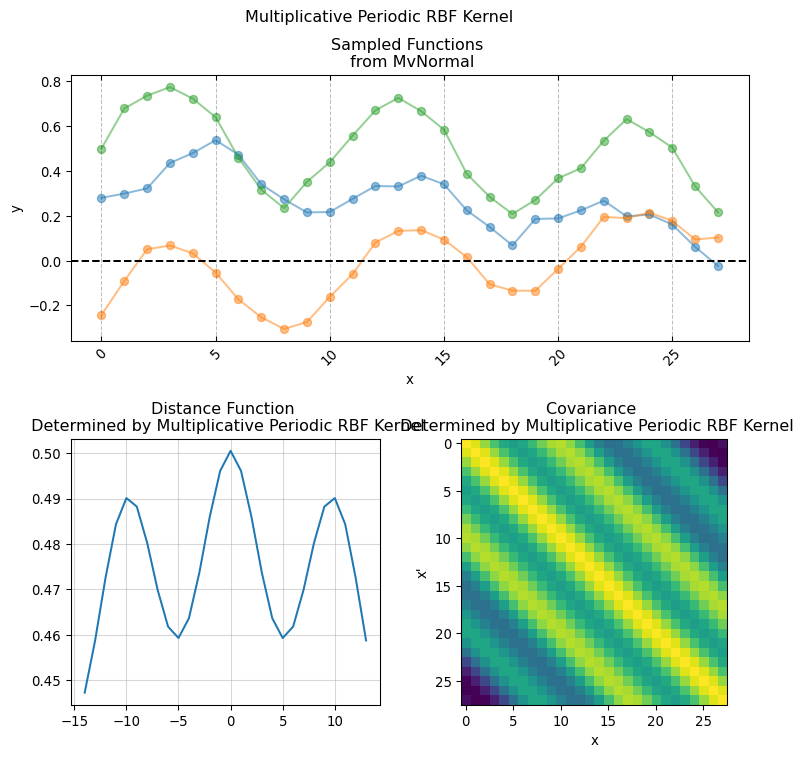
One convenient property of \(GP\) is that the sum and multiplication of two or more \(GP\) is itself a \(GP\), this allows to combine different types of Kernels for imposing specific structural constrains.
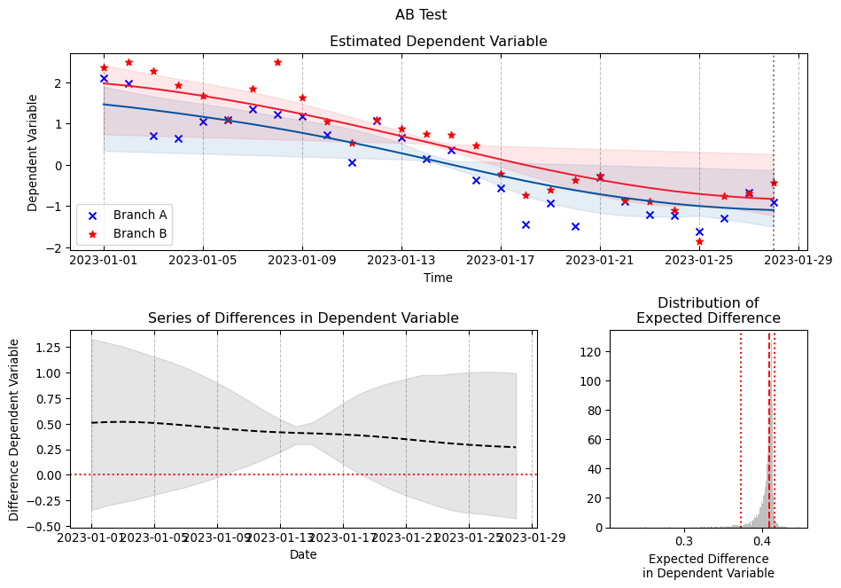
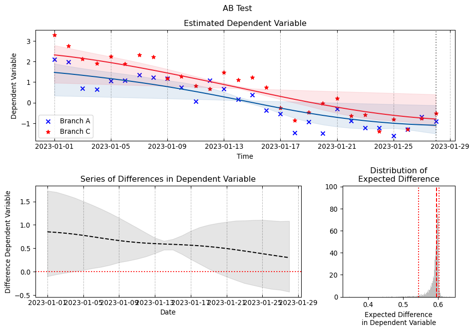
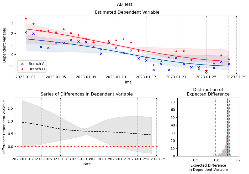
2.3 Gaussian Process for A/B test
Although we were not able to find many papers illustrating how \(GP\) can be used for analyzing A/B test data we found this interesting work by (Benavoli and Mangili 2015) from IDSIA that we decided to adapt to our use-case.
3 Implementing a Gaussian Process Model in Numpyro
In this section we will illustrate how we can implement a \(GP\) model using Numpyro. Numpyro offers a Numpy-like Backend for Pyro a Probabilistic Programming Language (PPL). Other than offering the flexibility of specifying models using the familiar Numpy interface, Numpyro is perfectly integrated with JAX allowing us to tap into its JIT compilation capabilities.
BLUE = (0, 83, 159)BLUE =tuple(value /255.for value in BLUE)RED = (238, 28, 46)RED =tuple(value /255.for value in RED)TIME_IDX = np.arange(7*4)DATES = pd.date_range( start="01-01-2023", periods=len(TIME_IDX)).valuesTIME ="date"MODELS = ["Branch A","Branch B","Branch C","Branch D","Branch E",]
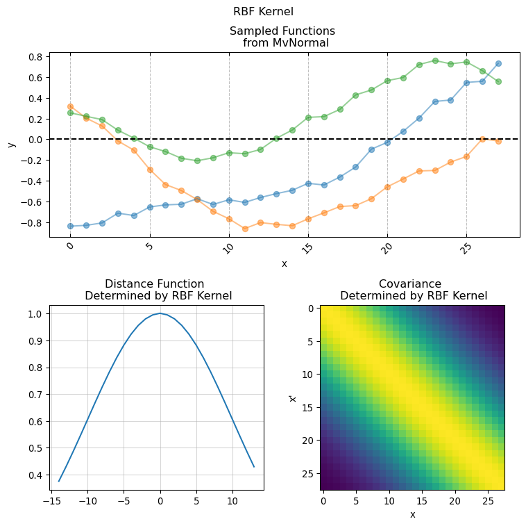
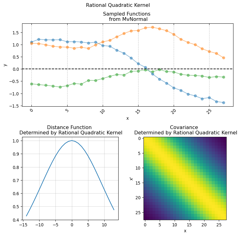
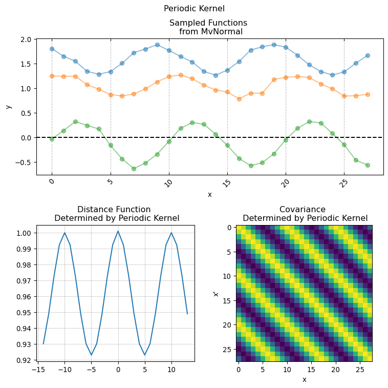
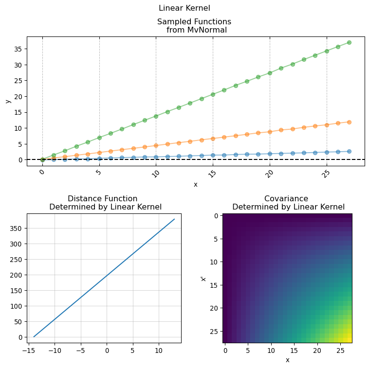
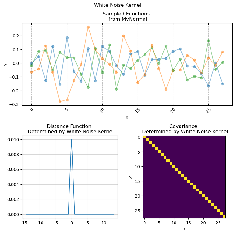
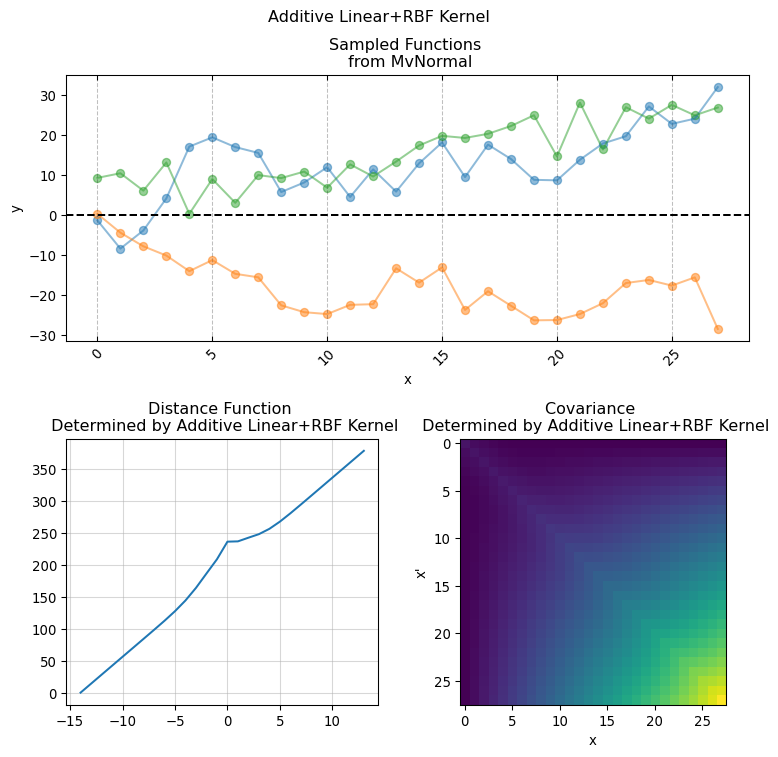
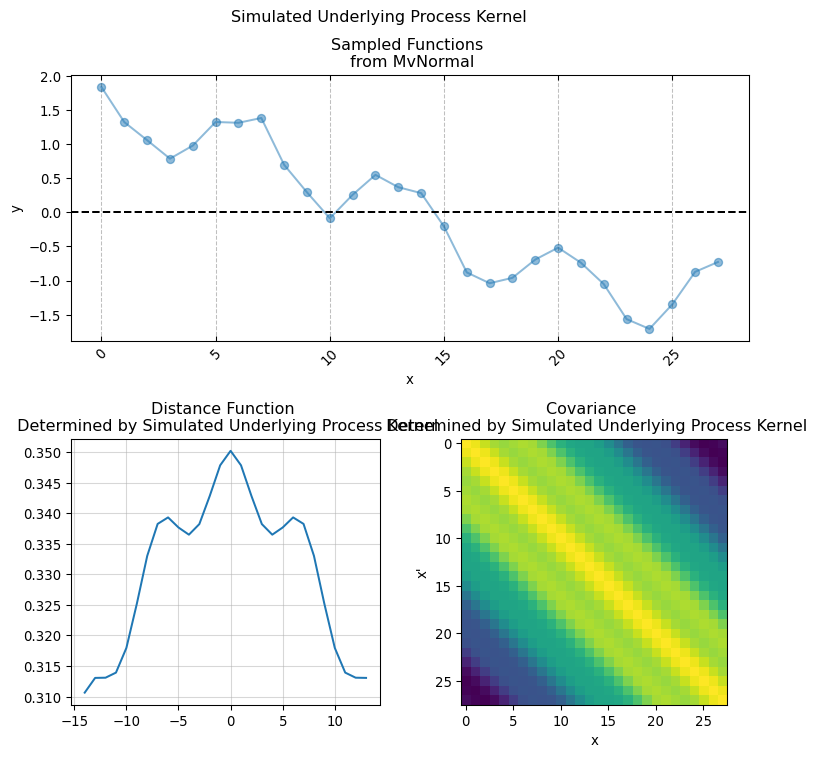
3.1 Kernel Functions
implementing Kernel functions in Numpyro is as easy as simply writing the functional form of the actual covariance function in pure python. It is sufficient that the python function has the following signature:
Here X and X_prime is the same input covariate used for creating the covariance matrix. While the keyword arguments are the parameters used for computing the pairwise relationship between each pair of of values in X (hence why we duplicate it using X_prime). This is the base for giving structure and creating our covariance matrix. We will now present a series of conventional covariance functions usually found in standard Gaussian Process applications.
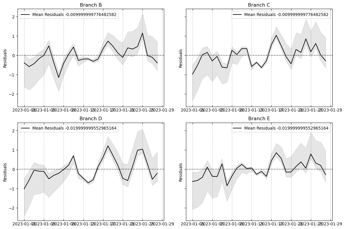
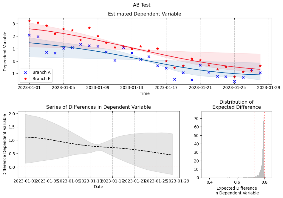
5 Fitting Gaussian Process Models to A/B test data
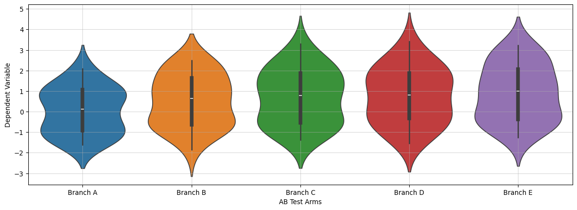
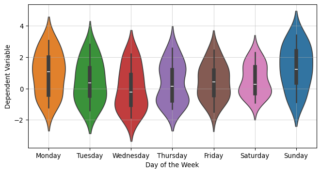
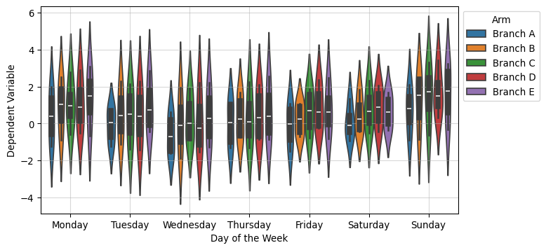
df = pd.DataFrame( simulated_series.T,# the names here indicates the 5 branches of an AB test. columns=MODELS)df["date"] = DATESdf["day_week"] = df["date"].dt.day_name()df.head()
from sklearn.preprocessing import OneHotEncodery_control = df["Branch A"].values.copy()y_models = { model_name: df[model_name].values.copy() for model_name in arms}( standardizing_mean, standardizing_std, y_control_standardized, y_models_standardized) = standardize_targets_to_common_statistics( reference_X=y_control, targets_X=y_models)# This can be read as the N of days over which the AB test was conductedX = np.linspace(0, 1, len(y_control))days = OneHotEncoder(sparse_output=False).fit_transform(df["day_week"].values.reshape(-1, 1))
Benavoli, Alessio, and Francesca Mangili. 2015. “Gaussian Processes for Bayesian Hypothesis Tests on Regression Functions.” In Artificial Intelligence and Statistics, 74–82. PMLR.
Duvenaud, David. 2014. “Automatic Model Construction with Gaussian Processes.” PhD thesis.
Gelman, Andrew, John B Carlin, Hal S Stern, and Donald B Rubin. 1995. Bayesian Data Analysis. Chapman; Hall/CRC.
Gelman, Andrew, Jennifer Hill, and Aki Vehtari. 2021. Regression and Other Stories. Cambridge University Press.
McElreath, Richard. 2018. Statistical Rethinking: A Bayesian Course with Examples in r and Stan. Chapman; Hall/CRC.