LinUCB for Contextual Multi-Armed Bandit

This post how to implement the Linear Upper Confindence Bound (Li et al. 2010) algorithm in JAX and applying it to a simulated contextual multi-armed bandit problem.

%load_ext watermark

from typing import Tuple, List, Any

from functools import partial

import numpy as np

from sklearn.datasets import make_classification
from sklearn.linear_model import LogisticRegression

from sklearn.manifold import TSNE

from jax.typing import ArrayLike
from jax.lax import scan
from jax import vmap
from jax import numpy as jnp
from jax import random, jit
from jax.scipy.linalg import inv

import matplotlib.pyplot as plt
from matplotlib.gridspec import GridSpec

@jit
def tempered_softmax(logits, temperature=1.):
    """Produce a tempered softmax given logits.

    Args:
        logits (ArrayLike): logits to be turned into probability.
        temperature (int, optional): parameter controlling the softness
        of the function, the higher the value the more soft is the function. 
        Defaults to 1.

    Returns:
        ArrayLike: simplex derived from the input logits.
    """
    nominator = jnp.exp(logits / temperature)
    denominator = jnp.sum(nominator, axis=1).reshape(-1, 1)
    return nominator / denominator

1 Premise

We want to stress how what is presented here is not at all novel but rather an exercise for leveraging the nice features that JAX offers and applying them for making the solution of a specific problem more efficient. Alot of credit for this post goes to the author of the original LinUCB paper, the contributors to the JAX library and to Kenneth Foo Fangwei for this very clear blogpost explaining the fundamentals of the algorithm.

1.1 What we will cover

1. Very brief introduction to multi armed and contextual multi armed bandit problems.
2. Very brief introduction to the LinUCB algorithm.
3. Simulating a disjoint contextual multi armed bandit problem.
4. Implementing the LinUCB algorithm in JAX.
5. Testing the algorithm on simulated data.
6. Accelerating testing and simulation using a GPU.
7. Evaluating the performance of the algorithm.

1.2 What we will not cover

1. JAX fundamentals.
2. In depth expalantion of multi-armed and contextual multi-armed bandit problems.
3. In depth expalantion of the LinUCB algorithm.

2 Introduction

2.1 Multi-Armed Bandit Problem

The multi-armed bandit problem describes a situation where an agent is faced with \(K = (k_0, k_1, \dots, k_n)\) different options (or arms), each one with an associated unknown payoff (or reward) \(r_k\)¹ (Sutton and Barto 2018).

The goal of the agent is to select, over a finite sequence of interactions \(T=(t_0, t_1, \dots, t_n)\), the set of options that will maximize the expected total payoff over \(T\) (Sutton and Barto 2018). What our agent is interested in then is the true value \(q*\) of taking an action \(a\) and selecting a given arm \(k\), the action associated with highest value should be the go-to strategy for maximizing the cumulative payoff

Since the true value is not known, our agent often has to rely on an estimate of such value which comes with an associated level of uncertainty. We can think of this in terms of the relationship between the mean of the distribution from which the rewards of a given arm are sampled and its empirical estimate with associated standard error.

Selecting the best set of actions over a finite number of interactions then requires a balance between and exploitative and explorative behaviour

1. Exploit the options with the highest associated estimated reward
2. Allow the exploration of other options in case our exploitative behaviour has been biased by noisy estimates.

2.2 Contextual Multi-Armed Bandit Problem

The conventional multi-armed bandit scenario attempts to solve what is called a non-associative task, meaning that the payoff of a given action (e.g. selecting one of the \(k\) available arms) doesn’t depend on any context. This means that as a measure of value for a given action, we are interested in

\(\mathbb{E}[r | K=k]\)

In a contextual multi-amred bandit scenario instead, the payoff of a given action is dependent on the context in which the action is performed. This implies that given a matrix of context vectors \(X_{K\times h}\) we try to estimate the value of a given action as

\(\mathbb{E}[r | K=k, X=x_k]\)

In order to get a better understanding of what we mean here, let’s simulate a potential generating process that could give rise to data suitable for a contextual multi-armed bandit problem.

2.2.1 Create the Simulation Dataset

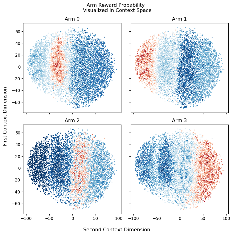
We will approximate the data generating process using sklearn’s make_classification function. The idea is to re-formulate this as a multi-class classification problem where the context are features able to influence the probability to pick one of n_arms classes.

In order to simulate some of the challenges we could face in a real world setting we will add the following hurdles:

1. Only a small portion of the features will actually have predictive power on which arm is the most promising.
2. We will generate features that have a certain degree of overlap (imagine them being drawn from relatively spread-out distributions)
3. We will enforce sparsity on the reward generated by each arm. This is like saying that the reward generated by pulling a given arm comes from a zero inflated distribution of the form

\[ \begin{gather} hurdle \sim Bernoulli(p_{hurdle}) \\ P(r | K=k, X=x_k) = \alpha x_k \\ r = \begin{cases} 0,& \text{if hurdle} = 0 \\ Bernoulli(p_{r}),& \text{otherwise} \end{cases} \end{gather} \]

UNIT_CONTEXT_SIZE = 1
UNIT_ARMS = 2

INFORMATIVE = 2
REPEATED = 0
REDUNDANT  = 0
RANDOM  = 8

CONTEXT_SIZE = INFORMATIVE + REPEATED + REDUNDANT + RANDOM

REWARD_SPARSITY = 0.99
REWARD_WEIGHTING = 1 / (1 - REWARD_SPARSITY)

N_USERS = 10000

N_ARMS = UNIT_ARMS ** 2 # We ensure we can always plot the arms in a squared grid
CLASS_SEP = .9

def generate_context(n_arms, n_users, context_size, redundant, repeated, informative, clusters_per_class, class_sep, with_intercept=True):
    context, groups = make_classification(
        n_classes=n_arms, 
        n_samples=n_users, 
        n_features=context_size,
        n_redundant=redundant,
        n_repeated=repeated,
        n_informative=informative,
        n_clusters_per_class=clusters_per_class,
        class_sep=class_sep
    )
    context = (context - context.mean(0)) / context.std(0)
    if with_intercept:

        context = np.hstack([context, np.ones(shape=(context.shape[0], 1))])
    
    return context, groups

def compute_arms_probabilities(context, groups, with_intercept=True, temperature=5):
    model = LogisticRegression(fit_intercept=not with_intercept).fit(context, groups)
    weights = model.coef_.T

    logits = context @ weights
    arms_probabilities = tempered_softmax(logits=logits, temperature=temperature)
    return arms_probabilities, model

def expand_context_to_arms(context, n_arms):
    context = np.array([context for _ in range(n_arms)])
    context = np.swapaxes(context, 0, 1)
    return context

CONTEXT, GROUPS = generate_context(
    n_arms=N_ARMS, 
    n_users=N_USERS, 
    context_size=CONTEXT_SIZE, 
    redundant=REDUNDANT, 
    repeated=REPEATED, 
    informative=INFORMATIVE, 
    clusters_per_class=1, 
    class_sep=CLASS_SEP, 
    with_intercept=True
)
ARMS_PROBAILITIES, MODE = compute_arms_probabilities(
    context=CONTEXT,
    groups=GROUPS,
    with_intercept=True,
)

CONTEXT = expand_context_to_arms(
    context=CONTEXT,
    n_arms=N_ARMS,
)

Here we will use TSNE for projecting the multidimensional context space on a 2D plane, this should allow us to get a better intuition of what is going on. What we expect to see are separate spheres or regions (this depends on how much noise we encode in our context space) with different coloring depending on which arms they are associated with

embedding = TSNE().fit_transform(CONTEXT[:, 0, :])

fig, axs = plt.subplots(UNIT_ARMS, UNIT_ARMS, figsize=(8, 8), sharex=True, sharey=True)
axs = axs.flatten()
for arm in range(ARMS_PROBAILITIES.shape[1]):

    axs[arm].scatter(
        embedding[:, 0],
        embedding[:, 1],
        c=ARMS_PROBAILITIES[:, arm],
        s=1,
        cmap="RdBu_r"
    )
    axs[arm].set_title(f"Arm {arm}")

fig.supylabel("First Context Dimension")
fig.supxlabel("Second Context Dimension")
fig.suptitle("Arm Reward Probability \n Visualized in Context Space")
plt.tight_layout()
plt.show()

2.3 LinUCB Algorithm for a Multi-Armed Bandit Problem

To solve a multi-armed bandit problem with context we can leverage an algorithm called Linear Upper Confidence Bound [li2010contextual] (i.e. LinUCB).

The aim of the algorithm is to progressively obtain a reliable estimate of all the options provided by the multi-armed bandit and to do so efficiently (i.e. with the smallest number of interactions.)

For doing so LinUCB simply fit a multinomial regression to the context (i.e. the covariates) provided by each arm of the bandit in order to estimate the return value associated with each arm, more formally

\[ \mathbb{E}[r_{t,k} | x_k] = x^\intercal \theta^*_k \tag{1}\]

where \(\theta^*_k\) are the set of parameters associated with a given arm \(k\) for which the algorithm is trying to find the optimal estimate. Here we assume \(x_k\) to be invariant across all \(t \in T\) but that is not always the case.

As the number of covariates can be large we cannot know a-priori if all of them are informative or if they are collinear. For this reason LinUCB rely on a form of regularized regression called Ridge Regression. Moreover since we don’t have a dataset to fit this model on but rather we refine the estimate for \(\theta^*_k\) as we interact with the arms \(K\), LinUCB utilizes what is called online learning for obtaining estimates of each interaction as given by

\[ \begin{gather} \mathbb{A}_k = \mathbb{X}_k^\intercal \mathbb{X_k} + \mathbb{I}_d\\ \hat{\theta_k} = \mathbb{A}^{-1}\mathbb{X}_k^\intercal r_k \end{gather} \]

where \(\mathbb{X}_k\) is the design matrix \(m \times d\) where \(m\) is the number of contexts (i.e., training inputs) and \(d\) the dimensionality of each context (i.e., the number of covariates considered). Here \(\mathbb{I}\) is the \(d\times d\) identity matrix and \(r_k\) is the corresponding \(m\)-dimensional reward (or response) vector. The identity matrix (which is usually expressed with a scaling factor \(\lambda\) here implicitly set to 1.) act as a constrain on the parameter \(\theta_k\).

The advantages of relying on the Ridge regression is that we can interpret \(\hat{\theta_k}\) a the mean of the Bayesian posterior of the parameter estimate and \(\mathbb{A}_k^-1\) its covariance. In this way we can compute the expectation for \(r_{t, k}\) as in Equation 1 and with it its associated standard deviation \(\sqrt{x_k^\intercal \mathbb{A_k}^{-1}x_k}\) which is proven to be a reasonable tight bound.

Based on this assumption then at any step \(t\) we can select the appropriate arm \(k\) to be

\(k_t = \arg \max_{k_t \in K_t}(x^\intercal \hat{\theta}_k + \alpha \sqrt{x_k^\intercal \mathbb{A_k}^{-1}x_k})\)

where \(\alpha\) becomes a constant that controls the exploration vs exploitation behaviour of the algorithm. Indeed, we can think of this as taking the value sitting at \(\alpha\) standard deviation at the right of the mean of a gaussian as most optimistic retun value when picking a certain arm. Larger values of \(\alpha\) will therefore encourage to select arms with highest UCB even if the return is much more uncertain (as the UCB lies far away from the expected value).

The positive aspect of this is that the more an arm get selected the tighter it’s confidence bound become, up to a point in which it will become more promising to explore arms that provides larger UCB by the fact that they have simply been explored less.

3 Implementing the Algorithm

In this section we will proceeded at implementing the LinUCB algorithm, step-by-step using JAX for hardware acceleration.

3.1 Parameters Initialization

As a first step we will need to initialize the matrices for \(X\) and \(r\) from this point onward we will call them \(A\) and \(b\) as mentioned in [li2010contextual].

def init_matrices(context_size: int) -> Tuple[ArrayLike, ...]:
    A = jnp.eye(N=context_size)
    b = jnp.zeros(shape=(context_size, 1))
    return A, b

def init_matrices_for_all_arms(
        number_of_arms: int, 
        context_size: int,
    )  -> Tuple[ArrayLike, ...]:

    arms_A = []
    arms_b = []
    for _ in range(number_of_arms):

        A, b = init_matrices(context_size=context_size)
        arms_A.append(A)
        arms_b.append(b)

    arms_A = jnp.array(arms_A)
    arms_b = jnp.array(arms_b)

    return arms_A, arms_b

3.2 Computations

We will now define the code for the various computations, namely deriving the \(\theta\) and \(\sigma\) parameters. And subsequently estimating the expectation for the return as well as the UCB.

In order to speed up the computation, we will leverage the Just in Time Compilation functionality in JAX as well as its automatic vectorization.

The first one will allow us to cache computations that are used multiple times by the LinUCB algorithm, while the second one will allow us in this case to vectorize the computation across all the arms in our bandit problem (instead of slowly iterating through them).

@jit
def compute_theta(
        A_inverse: ArrayLike, 
        b: ArrayLike,
    ) -> ArrayLike:

    theta = jnp.dot(A_inverse, b)
    return theta

@jit
def compute_sigma(
        context: ArrayLike, 
        A_inverse: ArrayLike,
    ) -> ArrayLike:

    sigma = jnp.sqrt(
        jnp.dot(
            jnp.transpose(context), 
            jnp.dot(A_inverse, context)
        )
    )
    return sigma

@jit
def compute_mu(
        theta: ArrayLike, 
        context: ArrayLike,
    )-> ArrayLike:

    mu = jnp.dot(
        jnp.transpose(theta),
        context
    )
    return mu

@jit
def compute_upper_bound(
        A: ArrayLike, 
        b: ArrayLike, 
        context: ArrayLike, 
        alpha: float,
    ) -> ArrayLike:
    A_inverse = inv(A)
    context_column = jnp.reshape(a=context, shape=(-1, 1))

    theta = compute_theta(
        A_inverse=A_inverse, 
        b=b
    )
    sigma = compute_sigma(
        context=context_column, 
        A_inverse=A_inverse
    )
    mu = compute_mu(
        theta=theta, 
        context=context_column
    )
    upper_bound = mu + (sigma * alpha)
    return upper_bound

@jit
def execute_linucb(
        alpha: float, 
        arms_A: ArrayLike, 
        arms_b:ArrayLike, 
        context: ArrayLike, 
        noise: ArrayLike,
    ) -> ArrayLike:
    partialized_compute_upper_bound = partial(
        compute_upper_bound,
        alpha=alpha
    )
    upper_bound = vmap(
        fun=vmap( 
            fun=partialized_compute_upper_bound, 
            in_axes=(0, 0, 0)
        ),
        in_axes=(None, None, 0)
    )(arms_A, arms_b, context).squeeze()
    upper_bound += noise
    return upper_bound

3.3 Update parameters

This section define the code used for updating the parameters associated with each of the arms, this function will be called dynamically during the simulation and will update the arms specified by the policy selected by the algorithm with the reward associated with said policy.

@jit
def update_parameters(
    arms_A: ArrayLike, 
    arms_b: ArrayLike, 
    arms_context: ArrayLike, 
    policy: ArrayLike, 
    reward: ArrayLike
) -> Tuple[ArrayLike, ArrayLike]:
    new_A=arms_A[policy, :, :] 
    new_b=arms_b[policy, :, :]
    context=arms_context[policy, :]

    context_column = jnp.reshape(a=context, shape=(-1, 1))
    new_A += jnp.dot(context_column, jnp.transpose(context_column))
    new_b += reward*context_column

    arms_A = arms_A.at[policy, :, :].set(new_A)
    arms_b = arms_b.at[policy, :, :].set(new_b)
    return arms_A, arms_b

4 Definining the simulation engine

Here we define all the functionality required for simulating the interactions with the various arms as well as the process of receiving rewards, executing the policies and updating the parameters. Also here, whenever possible, we will try to rely on the auto-vectorization and just-in-time compilation capacities provided by jax.

Since there is quite a bit to un-pack here, we will proceed step by step.

4.1 Taking a step in the simulation engine

In our case taking a step simply imply simulating the delivery of the reward from the arms selected by a given policy. Here we use policy interchangeably for indicating the strategy for selecting arms and the result of the selection itself.

The reward is simply given by sampling from a bernoulli distribution with its parameter $p$ defined by the arms_probabilities (the probability that a given arm will provide a reward). Since we want to makes this a bit more realistic, we will induce sparsity in the rewards by multiplying them with samples from another bernoulli distribution with parameter $p$ defined by 1 - reward_sparsity. We also included a reward_weighting parameter for exploring how this could be used for overcoming the sparsity problem.

Note

Note the importance of the step_key argument which is required for executing stochastic behaviors in JAX. More details can be found int the documentation about the stateless random number generators.

@jit
def step(
        policy: ArrayLike, 
        arms_probabilities: ArrayLike, 
        step_key: ArrayLike, 
        reward_sparsity: ArrayLike,
        reward_weighting: float,
    ) -> ArrayLike:
    sparsity_key, reward_key = random.split(step_key)
    rows = jnp.arange(start=arms_probabilities.shape[0])

    sparsity_factor = random.bernoulli(
        key=sparsity_key,
        p=1 - reward_sparsity,
        shape=(arms_probabilities.shape[0],),
    ) * 1
    rewards = random.bernoulli(
        key=reward_key,
        p=arms_probabilities[rows, policy]
    ) * 1
    return (rewards * sparsity_factor) * reward_weighting

4.2 Executing the policies

Executing the policies simply boils down to selecting the arm given the upper_bound computed by the LinUCB algorithm. In our case that correspond to take the arg-max of the generated upper_bound. For having a comparison term, we also implemented a random policy that simply selects one of the available arms at random.

@jit
def execute_policies(
        upper_bound: ArrayLike, 
        random_arm_key: ArrayLike,
    ) -> Tuple[ArrayLike, ArrayLike]:
    random_policy  = random.choice(
        key=random_arm_key, 
        a=jnp.arange(upper_bound.shape[1]),
        shape=(upper_bound.shape[0],)
    )
    linucb_policy = upper_bound.argmax(axis=1)
    return linucb_policy, random_policy

Once we have defined the logic for our simulation step and policies, we simply have to cycle through these policies and evaluate what type of reward they would obtain.

@jit
def compute_rewards(
        linucb_policy: ArrayLike, 
        random_policy: ArrayLike, 
        arms_probabilities: ArrayLike, 
        reward_sparsity: ArrayLike, 
        reward_weighting: float,
        step_key
    ) -> ArrayLike:
    arms_rewards = []
    for policy in [linucb_policy, random_policy]:

        rewards = step(
            policy=policy, 
            arms_probabilities=arms_probabilities, 
            reward_sparsity=reward_sparsity,
            reward_weighting=reward_weighting,
            step_key=step_key
        )
        arms_rewards.append(rewards)

    return arms_rewards

An interesting metric to compute on top of the reward obtained by executing a given policy is the regret. Regret can be thought as the distance between the optimal behavior the one produced by a given policy. In our case we compute the regret as the difference between the reward probability associated with the optimal arm and the probability associate with the arm selected by every policy.

@jit
def compute_regrets(
        linucb_policy: ArrayLike, 
        random_policy: ArrayLike, 
        arms_probabilities: ArrayLike
    ) -> List[ArrayLike]:
    policies_regrets = []
    optimality = arms_probabilities.max(1)
    rows = jnp.arange(start=arms_probabilities.shape[0])
    for policy in [linucb_policy, random_policy]:

        regret = optimality - arms_probabilities[rows, policy]
        policies_regrets.append(regret)
    
    return policies_regrets

4.3 Running the simulation

At this point the only thing that is left to do for us is to combine every piece of logic together into a single simulated interaction:

1. Execute the LinUCB algorithm and obtain the Upper Confidence Bounds for all the arms.
2. Derive the selected arms executing the LinUCB and Random policies.
3. Compute rewards and regrets associated with the selected arms
4. Update the LinUCB parameters based on the obtained rewards.
5. Update a diagnostic dictionary for tracking information related with the simulation

We can notice that simulate_interaction receives many of the needed variables from a carry parameter, which is then re-built and returned at the end. This structure is necessary for leveraging JAX scan in place of an expensive for-loop.

The scan primitive allows us to JIT-compile the for loop without having to un-roll all the computations first (e.g., in case of 1000 iterations, this would have required JAX for first compile all the 1000 computations), which would have required a compilation time that grows as the square of the number of iterations. In our case we are using it for speeding up the compilation of the interactions-loop required for running the simulation.

@jit
def simulate_interaction(
        carry: Tuple[ArrayLike, ...], 
        x: Any, 
        arms_probabilities: ArrayLike, 
        alpha: float, 
        reward_weighting: float,
        reward_sparsity: float
    ) -> Any:
    split_key, arms_A, arms_b, context = carry
    noise_key, random_arm_key, step_key, split_key = random.split(split_key, 4)  
    noise = random.normal(
        key=noise_key, 
        shape=(context.shape[0], arms_A.shape[0])
    ) * 1e-5

    upper_bound = execute_linucb(
        alpha=alpha, 
        arms_A=arms_A, 
        arms_b=arms_b, 
        context=context, 
        noise=noise,
    )
    linucb_policy, random_policy= execute_policies(
        upper_bound=upper_bound, 
        random_arm_key=random_arm_key
    )
    linucb_rewards, random_rewards = compute_rewards(
        linucb_policy=linucb_policy, 
        random_policy=random_policy, 
        arms_probabilities=arms_probabilities, 
        reward_sparsity=reward_sparsity,
        reward_weighting=reward_weighting,
        step_key=step_key
    )
    linucb_regrets, random_regrets = compute_regrets(
        linucb_policy=linucb_policy, 
        random_policy=random_policy, 
        arms_probabilities=arms_probabilities
    )

    arms_A, arms_b = vmap(
        fun=update_parameters, 
        in_axes=(None, None, 0, 0, 0)
    )(arms_A, arms_b, context, linucb_policy, linucb_rewards)
    arms_A = arms_A.mean(0)
    arms_b = arms_b.mean(0)

    new_carry = (split_key, arms_A, arms_b, context)
    diagnostics = {
        "parameters": {"A": arms_A, "b": arms_b},
        "policies": {
            "linucb": {"rewards": linucb_rewards, "regrets": linucb_regrets}, 
            "random": {"rewards": random_rewards, "regrets": random_regrets}
        }

    }

    return new_carry, diagnostics

5 Running the simulation and visualizing the performance

We now have to simply run our simulation and visualize the results! A couple of clarification point howecver are needed

1. We generate a PRNG split_key which will then be feeded inside the simulation. This is very important as it is the root PRNG key which will generate all the others required for the stochastic behaviours in our code.

2. The return from scan is always made of two component, the carry and the “result”. Although the carry is “consumed” inside the function that is scanned, the result stacks as we would normally expect in a for python loop (e.g., if we scan over a 1000 elements we will obtain 1000 stacked results).

SIMULATION_STEPS = 10000

split_key = random.PRNGKey(666)
arms_A, arms_b = init_matrices_for_all_arms(
    number_of_arms=N_ARMS, 
    context_size=CONTEXT.shape[-1]
)
partialized_simulate_interaction = partial(
    simulate_interaction, 
    arms_probabilities=ARMS_PROBAILITIES, 
    alpha=1,
    reward_sparsity=REWARD_SPARSITY,
    reward_weighting=REWARD_WEIGHTING,
)
carry, diagnostics = scan(
    partialized_simulate_interaction, 
    init=(split_key, arms_A, arms_b, CONTEXT),
    xs=jnp.arange(SIMULATION_STEPS)
)

6 Performance Visualisation

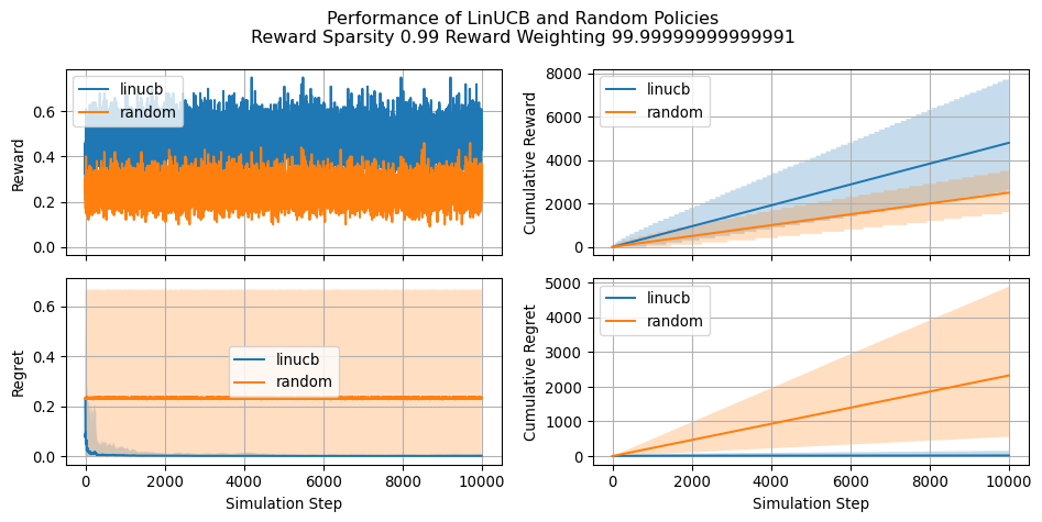
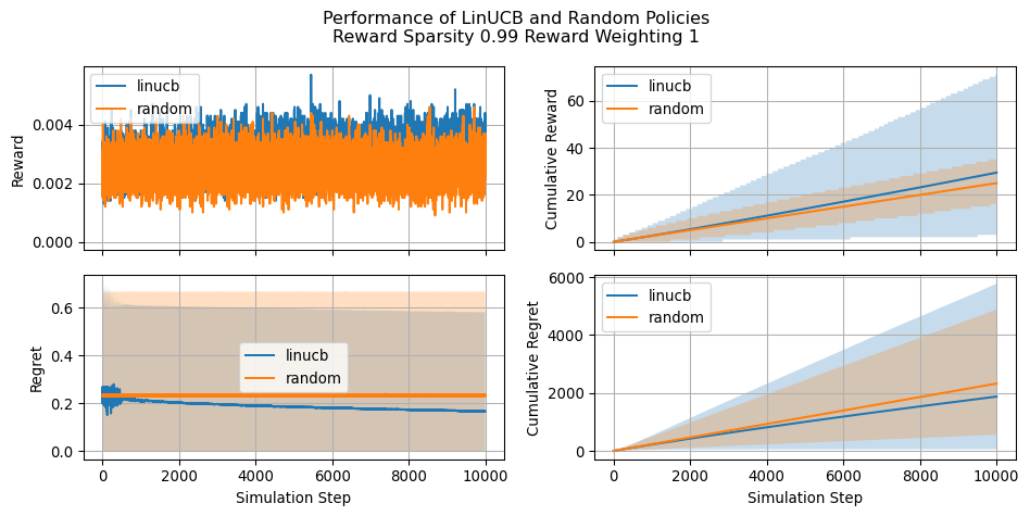
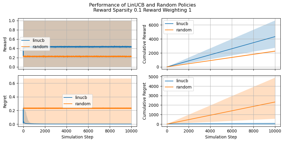
Let’s see now how our implementation of LinUCB compares against a naive random policy and how the estimated parameters changes during the simulation. Let’s keep in mind that greater (cumulative) reward indicates a more effective policy. Conversely, a lower cumulative regret is indicative of a better policy. We will see that regret becomes a particulary useful when asessing the performance in situations where reward is very sparse.

def compute_policy_diagnostics_summaries(diagnostics):
    diagnostics_summaries = {}
    for policy, diagnositcs_dict in diagnostics.items():

        diagnostics_summaries[policy] = {}

        for diagnostic, value in diagnositcs_dict.items():

            cumsum_value = value.cumsum(0)

            diagnostics_summaries[policy][diagnostic] = {
                "mean": value.mean(1), 
                "upper_percentile": np.percentile(value, 2.5, axis=1), 
                "lower_percentile": np.percentile(value, 97.5, axis=1), 
                "cumsum_mean": cumsum_value.mean(1), 
                "cumsum_upper_percentile": np.percentile(cumsum_value, 2.5, axis=1),
                "cumsum_lower_percentile": np.percentile(cumsum_value, 97.5, axis=1)
            }
    return diagnostics_summaries
 
def plot_policy_diagnositc(mean, lower_percentile, upper_percentile, ax, label):
    ax.plot(
        mean,
        label=label
    )
    ax.fill_between(
        x=np.arange(mean.shape[0]),
        y1=lower_percentile,
        y2=upper_percentile,
        alpha=0.25
    )
    return ax

def plot_all_policy_diagnostics(diagnostics_summaries, figsize=(10, 20)):
    fig, axs = plt.subplots(
        nrows=2, 
        ncols=2, 
        figsize=figsize, 
        sharex=True
    )
    axs = axs.flatten()

    for policy in list(diagnostics_summaries.keys()):

        ax = plot_policy_diagnositc(
            mean=diagnostics_summaries[policy]["rewards"]["mean"], 
            lower_percentile=diagnostics_summaries[policy]["rewards"]["upper_percentile"], 
            upper_percentile=diagnostics_summaries[policy]["rewards"]["lower_percentile"], 
            ax=axs[0], 
            label=policy
        )
        ax.set_ylabel("Reward")
        ax = plot_policy_diagnositc(
            mean=diagnostics_summaries[policy]["rewards"]["cumsum_mean"], 
            lower_percentile=diagnostics_summaries[policy]["rewards"]["cumsum_upper_percentile"], 
            upper_percentile=diagnostics_summaries[policy]["rewards"]["cumsum_lower_percentile"], 
            ax=axs[1], 
            label=policy
        )
        ax.set_ylabel("Cumulative Reward")

        ax = plot_policy_diagnositc(
            mean=diagnostics_summaries[policy]["regrets"]["mean"], 
            lower_percentile=diagnostics_summaries[policy]["regrets"]["upper_percentile"], 
            upper_percentile=diagnostics_summaries[policy]["regrets"]["lower_percentile"], 
            ax=axs[2], 
            label=policy
        )
        ax.set_ylabel("Regret")
        ax.set_xlabel("Simulation Step")
        
        ax = plot_policy_diagnositc(
            mean=diagnostics_summaries[policy]["regrets"]["cumsum_mean"], 
            lower_percentile=diagnostics_summaries[policy]["regrets"]["cumsum_upper_percentile"], 
            upper_percentile=diagnostics_summaries[policy]["regrets"]["cumsum_lower_percentile"], 
            ax=axs[3], 
            label=policy
        )
        ax.set_ylabel("Cumulative Regret")
        ax.set_xlabel("Simulation Step")

    for ax in axs:

        ax.grid()
        ax.legend()
    
    return fig

6.1 Visulize reward and regret performance

Since our simulation involves selecting the optimal arm for a large sampole of users (i.e. 10,000), we will alwways try to visualize expected reward and regret along with the 2.5 and 97.5 percentiles (the shaded are in the plot).

diagnostics_summaries = compute_policy_diagnostics_summaries(
    diagnostics=diagnostics["policies"]
)
fig = plot_all_policy_diagnostics(
    diagnostics_summaries=diagnostics_summaries, 
    figsize=(10, 5)
)
plt.suptitle(f"Performance of LinUCB and Random Policies\nReward Sparsity {REWARD_SPARSITY} Reward Weighting {REWARD_WEIGHTING}")
plt.tight_layout()
plt.show()

Let’s also have a look at how the simulation changes as we change the reward_sparsity and reward_weighting parameters

def run_parametrized_simulation(reward_sparsity, reward_weighting):
    split_key = random.PRNGKey(666)
    arms_A, arms_b = init_matrices_for_all_arms(
        number_of_arms=N_ARMS, 
        context_size=CONTEXT.shape[-1]
    )
    partialized_simulate_interaction = partial(
        simulate_interaction, 
        arms_probabilities=ARMS_PROBAILITIES, 
        alpha=1,
        reward_sparsity=reward_sparsity,
        reward_weighting=reward_weighting,
    )
    carry, diagnostics = scan(
        partialized_simulate_interaction, 
        init=(split_key, arms_A, arms_b, CONTEXT),
        xs=jnp.arange(SIMULATION_STEPS)
    )

    diagnostics_summaries = compute_policy_diagnostics_summaries(
        diagnostics=diagnostics["policies"]
    )
    fig = plot_all_policy_diagnostics(
        diagnostics_summaries=diagnostics_summaries, 
        figsize=(10, 5)
    )
    plt.suptitle(f"Performance of LinUCB and Random Policies\nReward Sparsity {reward_sparsity} Reward Weighting {reward_weighting}")
    plt.tight_layout()
    plt.show()
    return None

Here we maintain the same sparsity level but reduce the weighting (we basically introduce no weighting)

run_parametrized_simulation(
    reward_sparsity=REWARD_SPARSITY, 
    reward_weighting=1
)

While in here we reduce the sparsity of the reward and maintain that weighting at 1:

run_parametrized_simulation(
    reward_sparsity=.1, 
    reward_weighting=1
)

6.2 Visulize Parameters Evolution

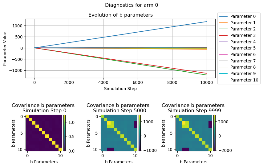
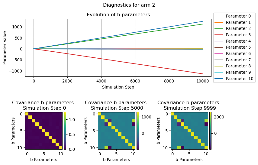
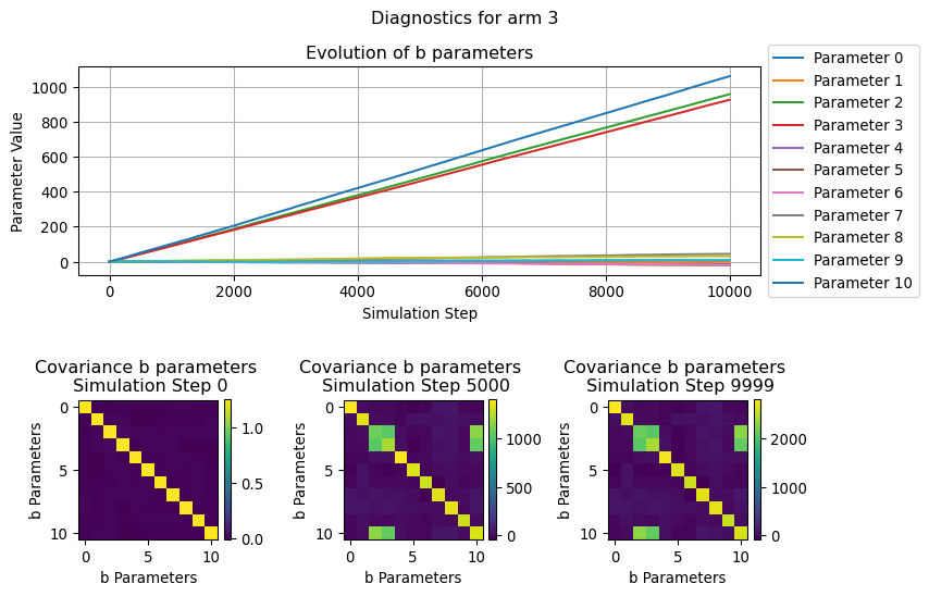
In this section we will visualize how the parameters used by the LinUCB algorithms evolve over the simulation time, in particular we will focus on the b parameters.

Since this can be thought as the the coefficient of a (regularized) linear regression, we can see its evolution for each of the considered arm as the “relevance” that a given covariate in a context has in determining the likelyhood of receiveing a reward.

Similarly, the evolution of the covariance illustrate how the relationship between the various b parameters change over the simulation steps.

def plot_single_arm_parameters_dianoistics(arm, diagnostics, figsize, show_labels=True):
    fig = plt.figure(figsize=figsize, tight_layout=True)
    grid = GridSpec(nrows=2, ncols=3)

    beta = diagnostics["b"][:, arm, :].squeeze()
    midpoint = int(beta.shape[0] // 2)
    simulation_steps = np.arange(beta.shape[0])

    ax_beta = fig.add_subplot(grid[0, :])
    for parameter_index in np.arange(beta.shape[-1]):

        ax_beta.plot(
            beta[:, parameter_index],
            label=f"Parameter {parameter_index}"            
        )
    
    if show_labels:
        ax_beta.legend(loc='center left', bbox_to_anchor=(1, 0.5))
    ax_beta.set_ylabel("Parameter Value")
    ax_beta.set_xlabel("Simulation Step")
    ax_beta.set_title("Evolution of b parameters")
    ax_beta.grid()

    for column, simulation_step in enumerate(simulation_steps[[0, midpoint, -1]]): 

        ax_alpha = fig.add_subplot(grid[1, column])
        ax_alpha.set_ylabel("b Parameters")
        ax_alpha.set_xlabel("b Parameters")
        ax_alpha.set_title(f"Covariance b parameters \n Simulation Step {simulation_step}")
        
        
        alpha_img = ax_alpha.imshow(
            diagnostics["A"][simulation_step, arm, :, :]
        )
        plt.colorbar(
            alpha_img,
            ax=ax_alpha,
            fraction=0.046, 
            pad=0.04
        )
    
    plt.suptitle(f"Diagnostics for arm {arm}")
    
    return fig

for arm in range(N_ARMS):

    fig = plot_single_arm_parameters_dianoistics(
        arm=arm, 
        diagnostics=diagnostics["parameters"], 
        figsize=(9, 6)
    )
    plt.show()

7 Conclusion

In this post we provided a brief overview of the LinUCB algorithm and illustrated how to implement it using JAX for speeding up computations. We saw how LinUCB resulted effective when compared with a random policy even in situation of extremely high reward sparsity. We also saw how applying weighting to the reward signal is an effective strtegy for mitigating said sparsity.

8 Hardware and Requirements

Here you can find the hardware and python requirements used for building this post.

%watermark

Last updated: 2025-03-29T13:18:45.106569+00:00

Python implementation: CPython
Python version       : 3.13.2
IPython version      : 9.0.2

Compiler    : Clang 18.1.8 
OS          : Darwin
Release     : 24.3.0
Machine     : arm64
Processor   : arm
CPU cores   : 14
Architecture: 64bit

%watermark --iversions

sklearn   : 1.6.1
matplotlib: 3.10.1
jax       : 0.5.2
numpy     : 2.2.4

References

Li, Lihong, Wei Chu, John Langford, and Robert E Schapire. 2010. “A Contextual-Bandit Approach to Personalized News Article Recommendation.” In Proceedings of the 19th International Conference on World Wide Web, 661–70.

Sutton, Richard S, and Andrew G Barto. 2018. Reinforcement Learning: An Introduction. MIT press.

Footnotes

1. The assumption is that the payoff comes from a stationary distribution, meaning that at any point in time we can expect that \(r_k \sim \mathcal{N}(\mu_k, \sigma_k)\) (or any other suitable probability distribution).