2 - Model specification and fitting

This post introduces the general set-up that we will use in this tutorial for specifying models and fitting them to the data.

%load_ext watermark

import numpy as np
import matplotlib.pyplot as plt

from jax.debug import print as jprint

In order to specify models in JAX we first need to figure out what are the core functionalities that we need to implement. We will focus on specific set of models that given an input \(X\), a target \(y\) and parameters \(\theta\) aim to approximate functions of the form \(f(X; \theta) \mapsto y\).

What we need to specify are:

1. Parameters-related functionalities:
   • Storage, how to best keep records of our parameters.
   • Initialisation, how to set our parameters to good starting points.
   • Sharing, how to make the parameters available to the model.
2. Model-related functionalities:
   • Forward computations, how to move from an input to an estimate of the target.
   • Objective computations, how to define suitable loss function along with any regularizing penalties.
   • Backward computations, how to derive the gradient of the parameters with respect to the model’s objective.
3. Optimization-related functionalities:
   • Optimization routines, how to find the optimal values for the parameters using suitable algorithms.
   • Parameters update, how to use the information derived from the backward computations for updating the parameters.
   • Fitting routines, how to connect the input, model and the optimization routines.

We also need to make sure that while developing these functionalities we leverage the optimisations provided by JAX while avoiding its sharp edges.

1 Parameters-related Functionalities

1.1 Parameters Container

The ideal way for storing parameters would be to create an immutable data structure (e.g., the named tuple example presented in our first post), registered as a pytree node, every time we need to update our parameters.

In this and future posts we will adopt a much simpler although more intuitive strategy and store our parameters in a dictionary.

from jax import numpy as jnp

my_parameters = {}

The nice thing about dictionaries is that they are:

1. Natively supported as a pytree.
2. Easy to inspect.
3. Naturally support nested structures.
4. Easy to update using native JAX functionalities

my_parameters["alpha"] = 1.

# more complicated structure
my_parameters["beta_1"] = {
    0: jnp.arange(5),
    1: jnp.arange(5, 10),
    2: jnp.arange(10, 15)
}
my_parameters["beta_2"] = {
    0: {
        "beta_21": jnp.arange(5),
        "beta_22": jnp.arange(5, 10),
        "beta_23": jnp.arange(10, 15)
    },
    1: 4.,
    2: 5.
}

1.2 Parameters Initialisation

One of the first step when fitting a model to the data is to set the starting point for the optimization process for each of the considered parameters.

We can achieve this by defining functions that implement specific initialisation strategies

def ones(init_state, random_key):
    """Initialise parameters with a vector of ones.

    Args:
        init_state (Tuple): state required to
        initialise the parameters. For this initializer only the parameters shape is required

        random_key (PRNG Key): random state used for generate the random numbers. Not used for this type of initialisation.

    Returns:
        param(DeviceArray): generated parameters
    """
    params_shape, _ = init_state
    params = jnp.ones(shape=params_shape)
    return params

one of the most straightforward strategies is to initialize all the parameters with the same constant value (a one in this case).

In this case we our function requires an init_state tuple containing all the information necessaries for initializing the parameters and a random_key used for setting the state of the random number generator. In this case we really do not need any random behaviour but we keep the signature for keeping compatibility with other initialisation strategies.

Another alternative is to generate starting values according to some statistical distribution, like a gaussian for instance

from jax.random import PRNGKey
from jax import random

import seaborn as sns

def random_gaussian(init_state, random_key, sigma=0.1):
    """Initialize parameters with a vector of random numbers drawn from a normal distribution with mean 0 and std sigma.

    Args:
        init_state (Tuple): state required to
        initialize the parameters. For this initializer only the parameters shape is required

        random_key (PRNG Key): random state used for generate the random numbers.

    Returns:
        param(DeviceArray): generated parameters
    """
    params_shape, _ = init_state
    params = random.normal(
        key=random_key,
        shape=params_shape
    ) * sigma
    return params

master_key = PRNGKey(666)

my_parameters = random_gaussian(
    init_state=((100, 2), None),
    random_key=master_key,
    sigma=0.1
    )

grid = sns.jointplot(
    x=my_parameters[:, 0],
    y=my_parameters[:, 1],
    kind="kde",
    height=4
)
grid.ax_joint.set_ylabel("Parameter 2")
grid.ax_joint.set_xlabel("Parameter 1")
plt.show()

1.3 Parameters Sharing

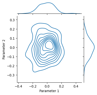
Sharing the parameters at this point is better understood as part of a state manipulation process. What do we mean by this? If we were to perform parameters update within a an object oriented framework we might do something among these lines

class Model:
    def __init__(self):
        self._parameters = np.array([0, 0, 0])

    def add(self, x):
        self._parameters += x

    def subtract(self, x):
        self._parameters -= x

    def get_parameters(self):
        return self._parameters

model = Model()
model.add(10)
model.subtract(5)

print(f"Updated Parameters {model.get_parameters()}")

Updated Parameters [5 5 5]

the parameters are part of the state of Model an get updated according to the behavior of add and subtract.

Since in JAX we have to stick to pure functions as much as we can, a viable option is to consider parameters as a state that is passed through a chain of transformation

from jax import jit

def parameters_init():
    return jnp.array([0., 0., 0.])

@jit
def add(parameters, x):
    return parameters + x

@jit
def subtract(parameters, x):
    return parameters - x

parameters = parameters_init()
# parameters are passed to transformations
# and returned modified
parameters = add(parameters=parameters, x=10.)
parameters = subtract(parameters=parameters, x=5.)

print(f"Updated Parameters {parameters}")

Updated Parameters [5. 5. 5.]

differently from the previous example, here the state (i.e., parameters) is made explicit and passed as argument to the functions in charge of doing the transformations.

2 Model-related Functionalities

Now that we have outlined how to generate, store and share parameters we must focus on the scaffolding describing the transformations performed by our model.

For the sake of simplicity we will use closures for being compliant with the functional requirements of JAX. We are aware that this might not be the optimal solution but it works just fine for the didactic purpose of this post. So let’s see how we would structure our closure

from jax import jit

def model(X, prng):

    @jit
    def init_params(X):
        pass

    @jit
    def forward(X, current_state):
        pass

    @jit
    def backward(X, y, current_state):

        @jit
        def compute_loss(y, y_hat):
            pass

        pass

    return init_params, forward, backward

In this case our model function would take a set of parameters (these are supposed to be constant and used by all the downstream functions) and return a collection functions in charge of performing parameters initialisation, forward and backward computations.

Let’s now go in more details of these specific functions.

2.1 Forward Computations

The forward function is in charge of performing all the the “forward computations” in the model. This naming, that we borrow from the various deep learning framework around, might not be the optimal one as we won’t necessarely need or have a complementary “backward” function but it is functional to the needs of this tutorial.

Let’s look at how the forward functiona for a simple linear model might look like

@jit
def forward(X, current_state):
    """Perform the forward computations for a linear model

    Args:
        x: covaruates of the model.
        current_state: current state of the model, containing 
        parameters and state for the pseudo random number generator.

    Returns:
        yhat: estimate of the target variable.
    """
    current_params, random_state = current_state
    beta = current_params["beta"]
    alphas = current_params["alphas"]
    yhat =  beta + jnp.dot(X, alphas)
    return yhat

Here, forward receive as input some data x and a variable we call current_state, as we see this last one it then gets unpacked in some current_parameters and a random_state. The idea here is that we are passing around the current state of the model (parameters or random number generator seed) instead of accessing it as we would with the attributes of a class.

Once unpacked all the necessary variables (here random state is spurious, but we could use it in case we need some stochastic behaviour from our function), the forward function simply execute all the logic necessary for mapping the input x to an estimate of our target variable yhat.

Once we obtain an estimate of our target variable, we should evaluate it with rispect to a given objective function, let’s see how we can do that with the compute_loss function.

2.2 Objective Computations

The computation of the objective function will require in our case four components: the parameters, the forward function, the loss function (along with any function used for computing any regularizing term) ad the input to the model.

We’ll see that we will pass all the components except the paramenters to the objective function using a closure and that the actual loss function need to be wrapped inside a compute_loss function.

from jax import tree_leaves

reg_strength = 0.001

X = np.random.normal(size=(100, 10))
y = np.random.normal(size=(100,))

params = {
    "alphas": np.random.normal(size=(10, )),
    "beta": np.random.normal(),
}

@jit
def root_mean_squared_error(y, yhat):
    """Compute the the root mean squared error between two vectors.

    Args:
        - y: ground truth value
        - yhat: estimate of ground truth
    
    Returns:
        squared_error: the squared mean error between y and y hat
    """
    squared_error = jnp.square(y - yhat)
    mean_squared_error = jnp.mean(squared_error)
    return jnp.sqrt(mean_squared_error)

@jit
def l1_reg_loss(params):
    """Compute the l1 norm of the parameters.

    Args:
        - y: ground truth value
        - yhat: estimate of ground truth
    
    Returns:
        squared_error: the squared mean error between y and y hat
    """
    loss = sum([jnp.sum(jnp.abs(leave)) for leave in tree_leaves(params)])
    return loss


def model(X, y, reg_strength):

    @jit
    def compute_loss(current_params):
        """Perform the computations required for deriving the loss given the current parameters.

        This inlcudes a call to the forward function, the loss computation and the regularisation
        loss.

        Args:
            current_params: the current state of the parameters of the model
        """
        yhat = forward(X=X, current_state=(current_params, None))
        raw_loss = root_mean_squared_error(y=y, yhat=yhat)
        reg_loss = l1_reg_loss(params=current_params) * reg_strength
        return raw_loss + reg_loss
    
    return compute_loss

/var/folders/h_/lq2hvf816xs9ffng6570sblh0000gn/T/ipykernel_3643/2913352642.py:1: DeprecationWarning: jax.tree_leaves is deprecated: use jax.tree.leaves (jax v0.4.25 or newer) or jax.tree_util.tree_leaves (any JAX version).
  from jax import tree_leaves

Of course there are are more intuitive ways for doing this but in this case we require this convoluted game of chinese boxes because when we apply the grad transformation we want it to give us the derivative of the objective function (root_mean_squared_error plus l1_reg_loss) with respect to the current_parameters. So in this case in order to obtain the derivative we can simple apply the relevant transformation value_and_grad to the compute_loss function

from jax import value_and_grad

compute_loss = model(X=X, y=y, reg_strength=reg_strength)
compute_loss_derivative = value_and_grad(compute_loss)

compute_loss_derivative(params)

(Array(4.255049, dtype=float32),
 {'alphas': Array([ 0.06140344, -0.09273863,  0.39737535,  0.13931032,  0.11116139,
         -0.5520289 ,  0.12071776,  0.1633386 ,  0.00850837,  0.00313382],      dtype=float32),
  'beta': Array(-0.65518194, dtype=float32, weak_type=True)})

What is particularly convinient in the functions defined above is the tree_leaves we use we computing the regularisation term. This utility function provided by jax allows us to traverse an antire PyTree in order to get all its leaves values, let’s see an example in action

complex_nested_pytree = {
    "a": (1, 2, 3),
    "b": 4,
    "c": {
        "c_1": 5,
        "c_2": 6,
        "c_3": {
            "c_3_1": 7,
            "c_3_2": 8,
            "c_3_3": 9
        }
    }
}

tree_leaves(complex_nested_pytree)

[1, 2, 3, 4, 5, 6, 7, 8, 9]

As you can see, this can become a convenient way for flattenting even the most intricate tree structure (such as those we have when specifying the parameters of a complex model).

2.3 Backward Computations

def model(X, y, reg_strength, loss_function, reg_function):

    @jit
    def backward(X, y, current_state):
        """Perform the backward computations for an arbitrary model defined by the forward function.

        For the most part backward is just a wrapper around compute_loss and forward which adds the 
        logic for computing the gradient of the loss wrt the current parameters.

        Args:
            X: covariates of the model.
            y: target of the model.
            current_pstate: current state of the model, containing 
            parameters and state for the pseudo random number generator.

        Returns:
            loss: loss computed on the forward pass
            grads: gradient of the loss wrt the model parameters.
        """

        @jit
        def compute_loss(current_state):
            """Perform the computations required for deriving the loss given the current parameters.

            This inlcudes a call to the forward function, the loss computation and the regularisation
            loss.

            Args:
                current_params: the current state of the parameters of the model
            """
            yhat = forward(X=X, current_state=current_state)
            raw_loss = loss_function(y=y, yhat=yhat)
            reg_loss = reg_function(params=current_state[0]) * reg_strength
            return raw_loss + reg_loss

        grad_func = value_and_grad(compute_loss)
        loss, grads = grad_func(current_state)
        return loss, grads

2.4 Optimizer

def newton_rhapson(learning_rate, beta=0.9):
    
    @jit
    def init_state(params):
        previous_updates = tree_map(lambda param: jnp.zeros_like(param), params)
        return previous_updates, params

    @jit
    def update_state(grads, current_state):
        previous_updates, previous_params = current_state
        current_updates = tree_map(
            lambda grad, previous_update: beta * previous_update
            + (grad * learning_rate),
            grads,
            previous_updates,
        )
        current_params = tree_map(
            lambda param, update: param - update, previous_params, current_updates
        )
        return current_updates, current_params

    @jit
    def get_params(state):
        current_update, current_params = state
        return current_params

    return init_state, update_state, get_params

3 Hardware and Requirements

Here you can find the hardware and python requirements used for building this post.

%watermark

Last updated: 2025-03-28T09:22:13.055626+00:00

Python implementation: CPython
Python version       : 3.13.2
IPython version      : 9.0.2

Compiler    : Clang 18.1.8 
OS          : Darwin
Release     : 24.3.0
Machine     : arm64
Processor   : arm
CPU cores   : 14
Architecture: 64bit

%watermark --iversions

jax       : 0.5.2
seaborn   : 0.13.2
matplotlib: 3.10.1
numpy     : 2.2.4